Preparing data for MaxEnt

There are two types of datasets required in MaxEnt; the species occurrence records and environmental covariates. Occurrence records are geographic points (i.e. coordinates) of species observation while environmental covariates are set of data that contains continuous or categorical values such as temperature, precipitation and land cover (for details see Pearson, 2007). To perform the modeling in MaxEnt, species occurrence should be in comma separated values (CSV) and covariates should be in raster Arc/Info ASCII Grid format.

The goal of this section is to guide you how to prepare these types of data using the occurrence records of Cebu black shama Copsychus cebuensis obtained from FFI and DENR field surveys on Cebu in 2012 and bioclimatic layers from WorldClim (http://www.worldclim.org/; Hijmans et al., 2005).

Species occurrence

Creating CSV file

1. Use a spreadsheet application (e.g. MS Office Excel or LibreOffice Calc) to encode the occurrence record. Make sure that coordinates are in geographic coordinates in decimal degrees.

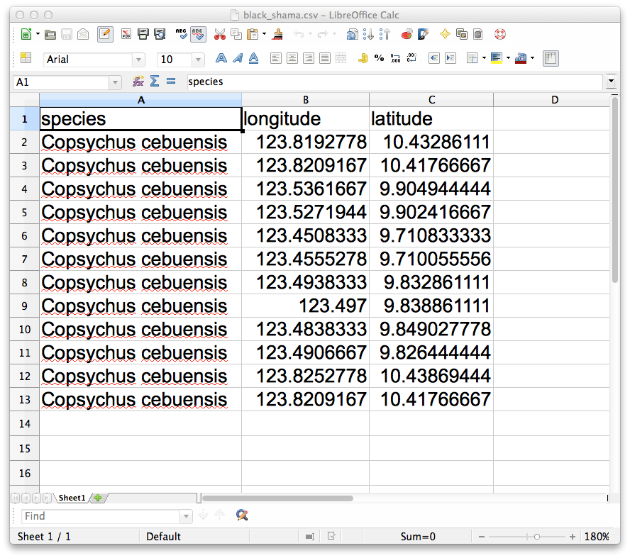
2. Format the occurrence record as shown below. Spreadsheet heading should be labeled as species, longitude and latitude.

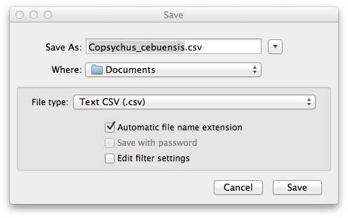
3. Convert the spreadsheet to CSV. In LibreOffice, select File ‣ Save As and choose Text CSV as the file type. Name the CSV file as Copsychus_cebuensis.csv and save it to your samples directory. The field delimiter should be comma (,).

The saved CSV file should look like the text below:

species,longitude,latitude
Copsychus cebuensis,123.8192778,10.43286111
Copsychus cebuensis,123.8209167,10.41766667
Copsychus cebuensis,123.5361667,9.904944444
Copsychus cebuensis,123.5271944,9.902416667
Copsychus cebuensis,123.4508333,9.710833333
Copsychus cebuensis,123.4555278,9.710055556
Copsychus cebuensis,123.4938333,9.832861111
Copsychus cebuensis,123.497,9.838861111
Copsychus cebuensis,123.4838333,9.849027778
Copsychus cebuensis,123.4906667,9.826444444
Copsychus cebuensis,123.8252778,10.43869444
Copsychus cebuensis,123.8209167,10.41766667

For multiple species, do the similar steps above and simply add other species after the first occurrence record.

Note

If data are recorded using a GPS device, it can be downloaded to QGIS using GPSBabel plugin and covert it directly to CSV format.

Checking and filtering occurrences

To ensure if the CSV file is working, it needs to be checked in QGIS. The records should also be checked to avoid potential bias of clustered points (Hernandez et al., 2006) and this can be done by removing duplicate records on each pixel.

1. Launch QGIS and load CSV using the Add delimited text layer.

If the plugin is not enabled, go to Plugins ‣ Manage Plugins. and check Add delimited text layer.

2. On Create a Layer from a Delimited Text file window, click Browse and select Copsychus_cebuensis.csv in the directory where the CSV is saved.

3. On the same window, choose Selected delimiters and check the Comma option. In the XY fields, select longitude as X and latitude as Y.

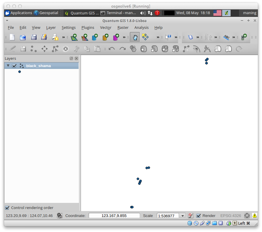
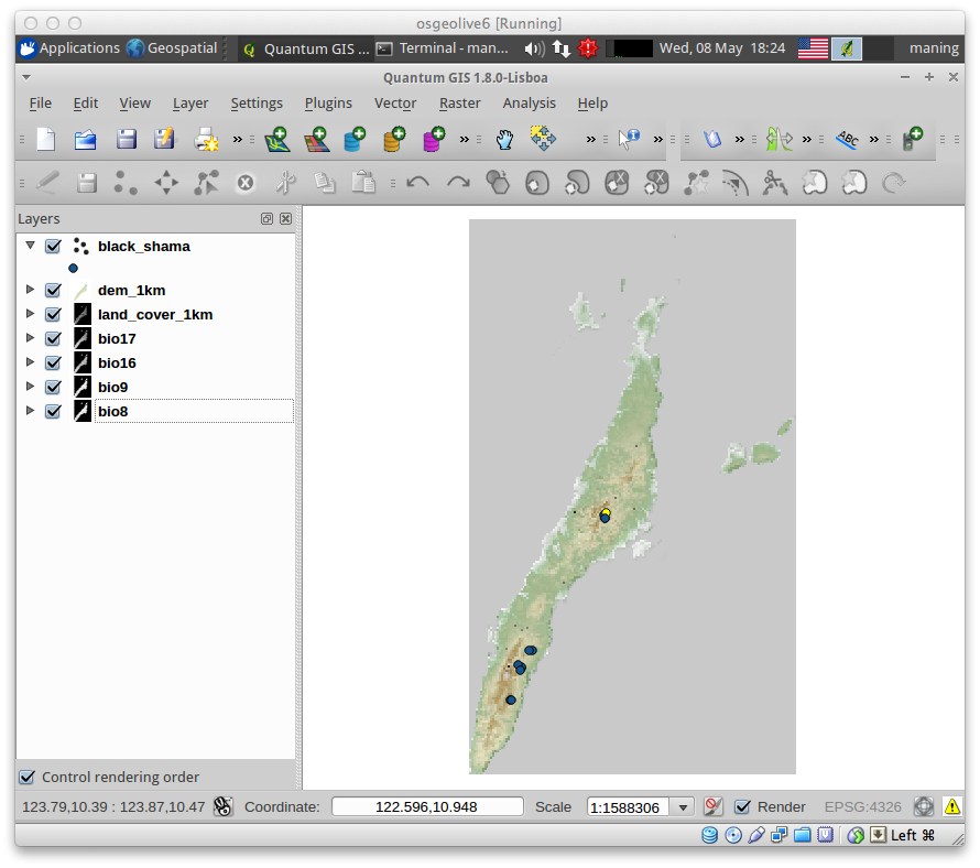
4. Click OK Select WGS-84 for the CRS and click OK, this should show the points in your Map View.

Note

The filtration of occurrences can be done depending on the resolution of your covariate raster layers. In this case, 1km resolution will be used. If you need a finer resolution for future studies, refer to image resampling section.

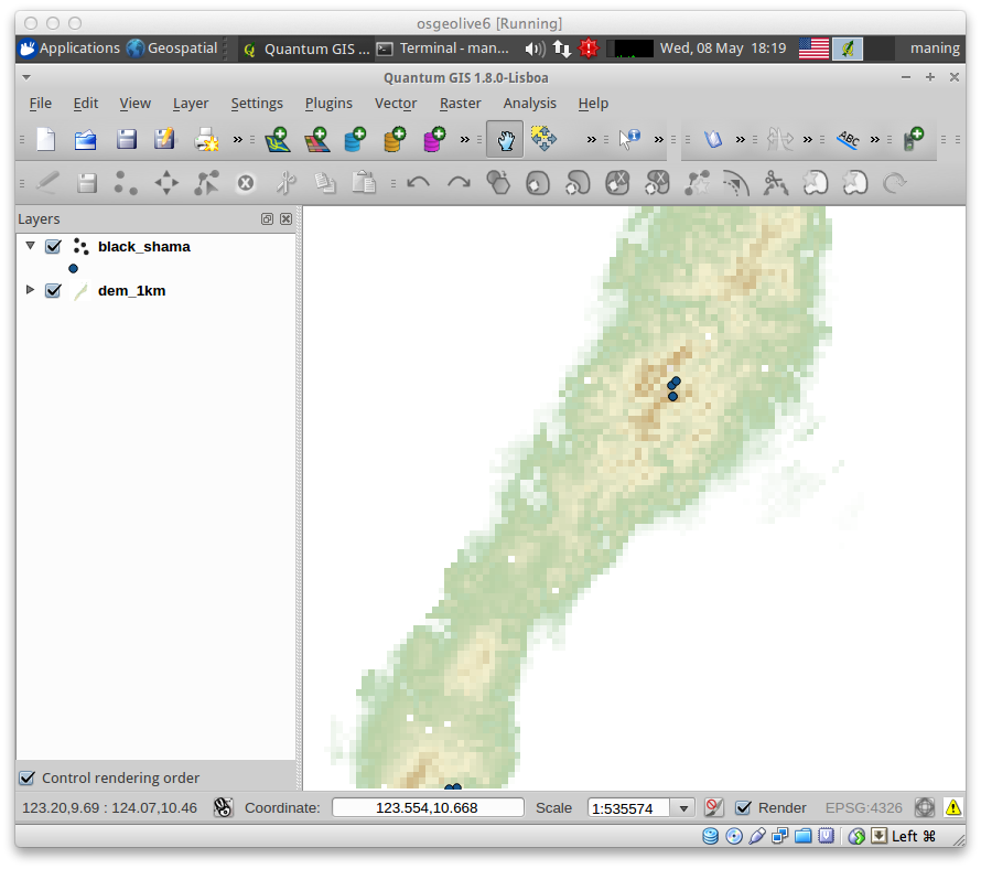
5. After importing the CSV to QGIS, load the dem_1km.asc raster you created previously. The elevation raster will be used as reference for filtration.

6. Use the navigation tool to move around the map and find the clustered occurrences. A clustered occurrence are 2 or more points that are within a single raster pixel.

7. Once clustered occurrences are found, select the species occurrence layer. Use the selection tool to select the identified clustered occurrences. Go to View ‣ Select ‣ Select single feature.

8. After selecting all the clustered occurrences, right click to occurrence layer. Select Properties and open Attribute Table.

Remember the selected occurrences and remove it in the CSV file by using either a text editor or a spreadsheet application.

Environmental Covariates

Data coming from various sources have different formats or spatial extent. For instance, many land cover (Hansen et al., 2000; Tateishia et al., 2001) or climate datasets (Hijmans et al.,) are done in global scale and because of data scarcity in local scale we tend to rely to what is available.

It is important for each environmental covariate layer to be in a consistent spatial extent, pixel size and data format.

Inspecting the raster environmental layers for data consistency

1. Add the rater environmental layers in QGIS. They are following:

   dem_1km.asc
   slope.asc
   bio8.asc
   bio9.asc
   bio16.asc
   bio17.asc
   landcover_1km.asc
   

Note

After loading the environmental layers to QGIS, always check the data information (i.e. metadata) because it will help you to understand how the data can be transformed to your desired format.

2. To check the metadata, select dem_1km.asc layer and right-click and select Properties and select Metadata tab on the Layer Properties window.

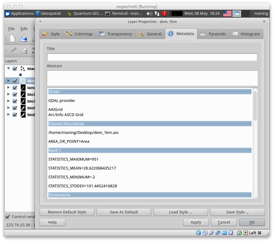
3. Make sure all the raster layers have the same spatial extent, size (1 km) number of pixel rows and columns, coordinate reference system (EPSG:4326 or WGS-84 and, data type (Int32).

4. If any layer is different, perform the resampling and format translation outlined in the previous section.

5. Once all the layers are in a uniform format, size and data type, make sure all layers are in one directory.