Using and Styling Rasters

QGIS can also display and manipulate raster data. These are available in Raster menu. In this section, we will customize the style of our Terrain or Digital Elevation Model (DEM) using the custom symbology and, create new raster and vector from the DEM.

Note

A Raster data is composed of rows (running across) and columns (running down) of pixels (also know as cells). Each pixel represents a geographical region, and the value in that pixel represents some characteristics of that region.

Images with a pixel size covering a small area are called ‘high resolution’ images because it is possible to make out a high degree of detail in the image. Images with a pixel size covering a large area are called ‘low resolution’ images because the amount of detail the images show is low.

Some raster data have two files included. For example, a file with the tif extension is the image and the file with the extension tfw is the world file. World files describe the location, scale and rotation of the map. By adding a world file in any image, GIS applications can read and georeference almost any image. However, the world file does not give the proper coordinate reference system of the raster. In QGIS, you have to properly set the CRS for raster with world file.

Loading a raster layer

1. Open your previously created QGIS project/session or create a new project.

2. Add the DEM raster. Select Layer ‣ Add Raster Layer and load the dem_90m.tif. Click OK.

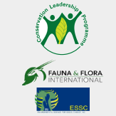
When the DEM is first loaded, it may appear as an entirely black square with some slight grayish colors showing up in some locations. This can be fixed by adjusting the stretch of the contrast enhancement to scale the shades of black and white to the values found within the data.

3. To adjust the contrast enhancement, select the dem_90m.tif, right-click and select Properties.

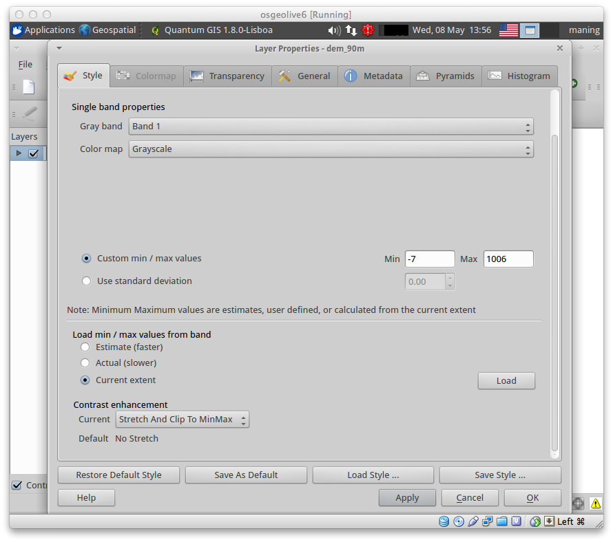
4. In the Style tab, change the Current value of Contrast Enhancement from No Stretch to Stretch And Clip to MinMax. In the Load min/max values from band, click the Load button.

This takes the minimum and maximum value found within the data, and stretches the black to white gradient between the two values.

A typical black to white gradient allows for 256 different levels of brightness, and stretching these 256 shades between the Min and Max values allows you to clearly view the different topography in the DEM data.

5. Click Apply and OK to improve the contrast of the layer.

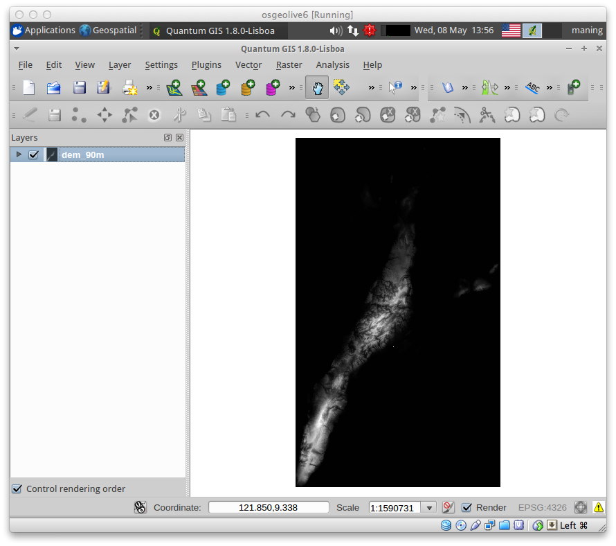
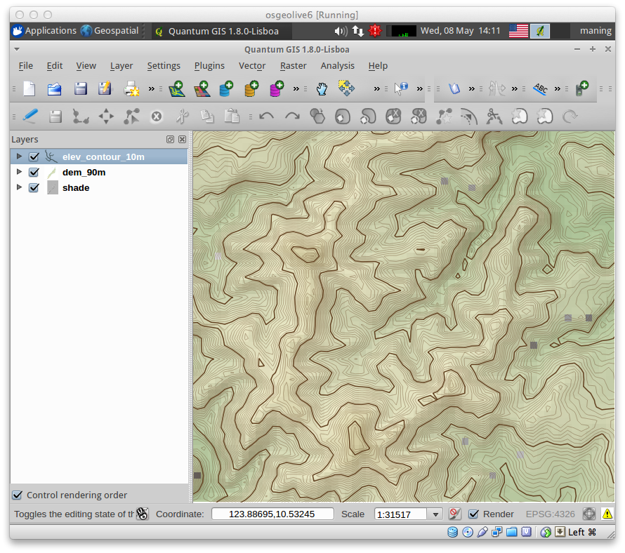
The enhanced contrast of layer shows a wide variation of pixel brightness values across the grid area, with dark black pixels representing areas of low elevation and bright white pixels representing areas of high elevation. To get the values for each pixel, use the Identify button.

Note

Terrain data is one of the most important data used in geospatial analysis. At the basic level, a terrain or surface is represented as: given a location (X,Y), the height or elevation (Z) is computed from a specific reference point.

Terrain data are represented in several of ways. Depending on the data source, it can be a set of points (Spot elevation) or lines (Contour). Within GIS, these data are modelled either as regular grids (known as Digital Elevation Model or Altitude matrix) or Triangular Irregular Network (TIN).

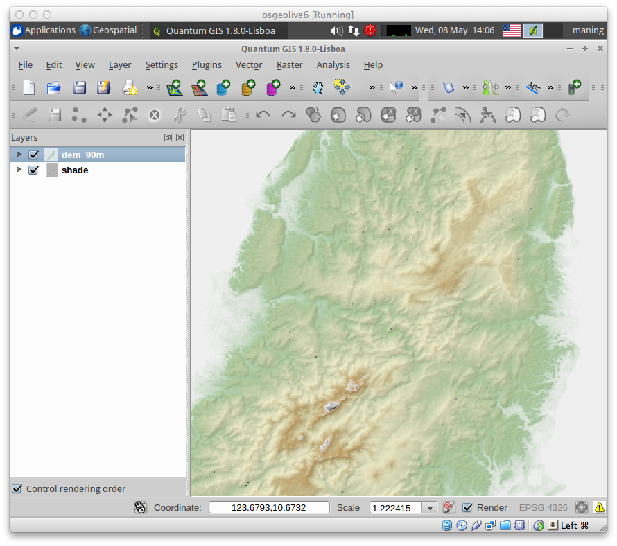
Using a custom color map for rasters

1. To use a custom color ramp for rasters, select the dem_90m.tif, right-click and select Properties.

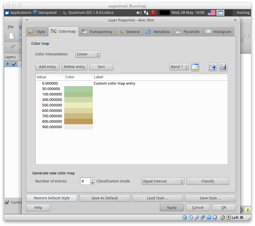
2. In the Style tab, choose Colormap in the Color map drop-down list.

3. To assign a new colormap, click the Colormap tab. Choose Linear in the Color interpolation drop-down list.

4. Click the Load style ... and use the dem.qml file in your data/styles directory.

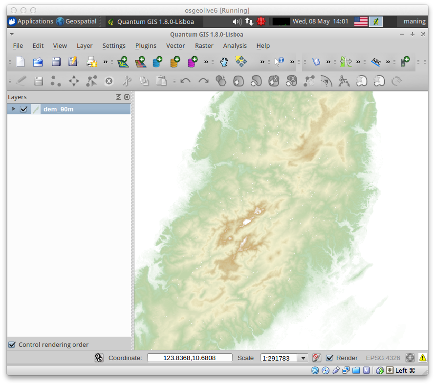
5. You can also adjust the layer transparency in the Transparency tab.

6. Finally, hit the OK to view the styled DEM in the Map View.

Loading the GDALTools plugin

1. Open the Plugin manager by selecting Plugins ‣ Manage Plugins.

2. Activate/enable the GDALTools plugin by clicking its check box or description.

Creating a shaded relief

With the GDALTools plugin, we will create a new relief layer using our DEM.

1. To create a new relief layers, select Raster ‣ Analysis ‣ DEM (Terrain Models).

A new window will appear for the DEM (Terrain Models) options.

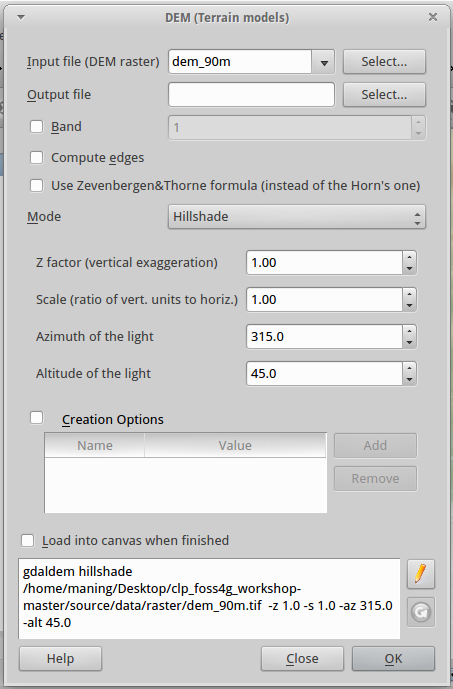
2. In the Output file, click Select and create a new layer as shade.tif.

3. In the Mode, select the Hillshade from the drop-down list.

4. Since we are using geographic coordinate system, we use a scale value of 111120. Type this value in the Scale field. We leave the other values to the default settings.

5. Put a check-mark in the Load into canvas when finished.

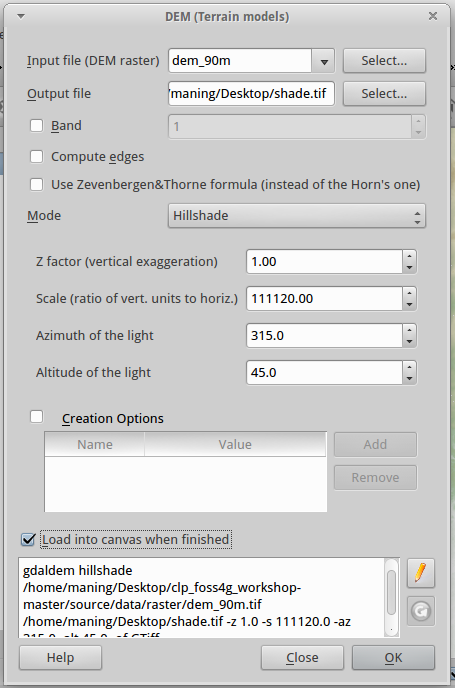
6. Finally, click the OK to begin the process. Close the GDALTools window when processing is completed.

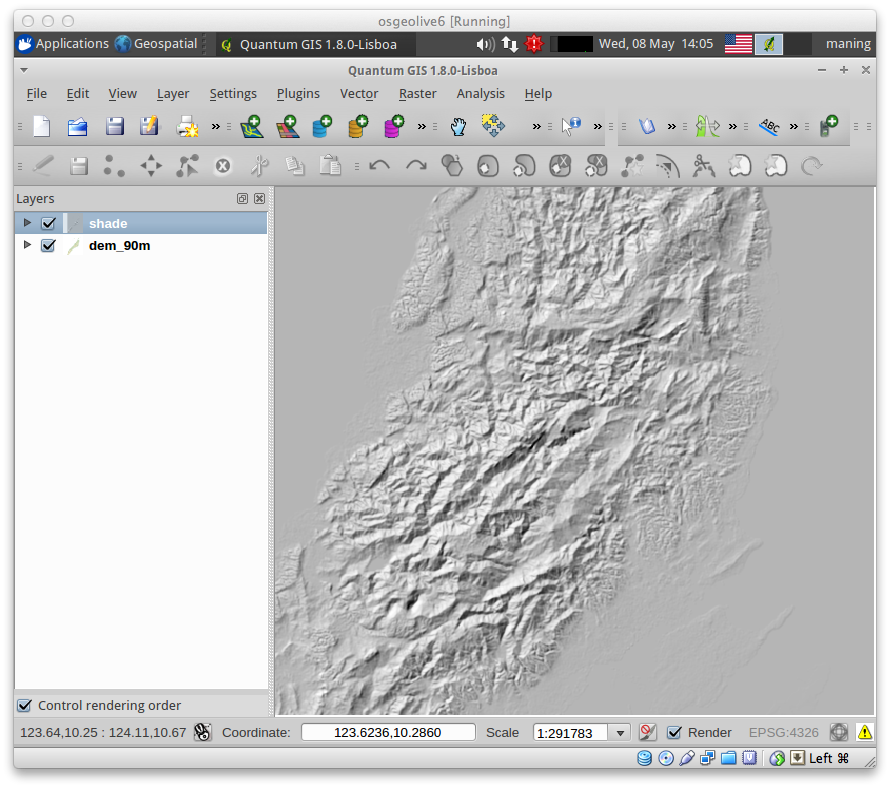
7. Move the shade layer below the dem layer to create shaded relief effect of the rendering.

The Shaded relief results provides the most visually appealing display of the DEM data. This analysis uses a fixed location of the sun and the horizon to accurately display areas of bright sun exposure as well as low dark areas that contain lots of shadow. Typically a shaded relief will be used in presentation of 3D GIS analysis as a thematic background layer that provides the user with pretty looking cartographic representation.

Tip

You can improve vertical exaggeration of the output hillshade by increasing the Z Factor value. A Z Factor of 5 to 7 increases the relief texture of the flatter areas.

8. Save you QGIS project.

Creating a vector contour

We can also extract elevation contour lines from our DEM.

1. To extract contour lines, select Raster ‣ Extraction ‣ Contour. A new window will appear for the Contour options.

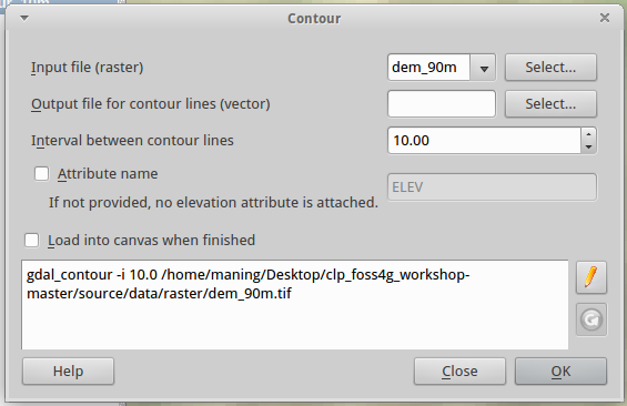
2. In the Output directory for contour lines, click Select and type elev_contour_20m in the File name.

3. Put a check-mark in the Attribute name and add elev (the default label was in upper-case, change it to lower-case) as the attribute name column.

4. Put a check-mark in the Load into canvas when finished.

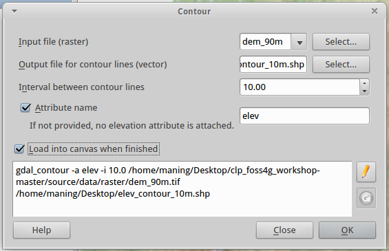
5. Finally, click the OK to begin the process. Close the GDALTools window when processing is completed.

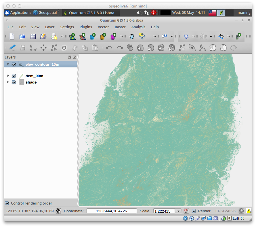
6. Improve on the look of your map by exploring the other style and symbology options. Save your project.